Styling R Code

01. What is code styling?

‘Styling’ covers…

Code/project structure (e.g. 01-modelling.R -> 02-plots.R -> 03-export.R )
Code formatting
- Naming things (variables, columns, functions etc)
- Indentation/line breaks/spacing
- Stuff specific to R, e.g. <- vs =
Wider principles like…
- What does a good comment say?
- What should a good function do?
Styling is about making your work easy to understand without changing its function

Good coding style is like correct punctuation: you can manage without it, butitsuremakesthingseasiertoread

-Introduction to the Tidyverse Style Guide

Some specific benefits

Styling makes writing code easier (less decisions to make)
Styling makes reading code easier
Styling makes it easier to avoid bugs

My styling journey

2019: Started coding in R
- Struggled to write clear code
- Often got frustrated by needing to rewrite stuff
2020-2021: Had some kind of set of conventions specific to myself
- Would occasionally change how I did something
- This made me dislike all the code I’d written previously
- This made me feel sad
2022: Started religiously following the Tidyverse style guide
- My code needed less rewrites
- I spent almost no time thinking about styling (just design)
- My code was clearer
- This made me feel happy
2023: Life is great

02. Some specific styling tips

Naming things

Keep names as short as you can while still being descriptive. Prioritise being descriptive!
Only use abbreviations in special cases, e.g. acronyms
Don’t use the name to signal the type of the object

Bad

table_totalcost <- costs %>% 
  group_by(Category) %>% 
  summarise(Cost = sum(Cost))

model_for_use_later_on <- lm(Cost ~ Time, data = costs)

read_data_func <- function(path) {
  readr::read_csv(path, id = "filepath", na = "N/A")
}

Good

cost_totals <- costs %>% 
  group_by(Category) %>% 
  summarise(Cost = sum(Cost))

cost_model <- lm(Cost ~ Time, data = costs)

read_data <- function(path) {
  readr::read_csv(path, id = "filepath", na = "N/A")
}

Names for things like dataframes, vectors, values etc should be noun-like, e.g. costs, costs_summary, costs_uplift_factor etc
Names for functions should be verb-like, e.g. filter(), standardise_names() , extract_coefficients() etc

Name case

# snake_case
iris_summary <- summary(iris)

# Title_Snake_Case
Iris_Summary <- summary(iris)

# camelCase
irisSummary <- summary(iris)

# PascalCase
IrisSummary <- summary(iris)

# SCREAMING_SNAKE_CASE
IRIS_SUMMARY <- summary(iris)

Consistency should be prioritised above all else, but…
lower_snake_case should be preferred in most cases
Title_Snake_Case works well for column names
You might see camelCase in other packages, but you shouldn’t use it unless you’re doing serious object-oriented programming

Syntactic names

R has rules for names:

They must only include letters and numbers _ and ., and must start with a letter or .
Other names must be surrounded by backticks:

# Good ('syntactic')
iris_proportions <- mutate(iris, across(1:4, ~ . / sum(.)))

# Bad: starts with a number
`01_iris_proportions` <- mutate(iris, across(1:4, ~ . / sum(.)))

# Bad: contains a non-alphanumeric character
`iris_%s` <- mutate(iris, across(1:4, ~ . / sum(.)))

# Bad: contains a space
`iris proportions` <- mutate(iris, across(1:4, ~ . / sum(.)))

When your data has non-syntactic column names, clean these up ASAP!
While names like my.data are allowed, avoid this naming style. Use my_data instead.

Indentation

Question: Why indent?
Answer: Indentation shows code structure at a glance
Whenever you increase indentation, do it by exactly 2 spaces
This usually means that all function arguments should have their own line

Bad

 iris %>% 
 dplyr::mutate(Sepal.Area = Sepal.Width * Sepal.Length,
   Petal.Area = Petal.Width * Petal.Length) %>% 
  ggplot2::ggplot(aes(x = Sepal.Area, 
y = Petal.Area, colour = Species)) +
  ggplot2::geom_point()

Better

iris %>% 
  dplyr::mutate(Sepal.Area = Sepal.Width * Sepal.Length,
                Petal.Area = Petal.Width * Petal.Length) %>% 
  ggplot2::ggplot(aes(x = Sepal.Area, 
                      y = Petal.Area, 
                      colour = Species)) +
  ggplot2::geom_point()

Best

iris %>% 
  dplyr::mutate(
    Sepal.Area = Sepal.Width * Sepal.Length,
    Petal.Area = Petal.Width * Petal.Length
  ) %>% 
  ggplot2::ggplot(aes(
    x = Sepal.Area, 
    y = Petal.Area, 
    colour = Species
  )) +
  ggplot2::geom_point()

Comments: what should they say?

Question: How much should you comment?
Answer: As much as needed, but no more

If a comment is needed, it should explain the why, not the what/how (if what your code does isn’t clear, you should probably rewrite it).

Bad

plot_data <- mtcars %>% 
  rownames_to_column("car") %>% 
  as_tibble() %>% 
  
  # Reorder car levels by values of mpg
  mutate(
    car = fct_reorder(car, mpg)
  )

Good

plot_data <- mtcars %>% 
  rownames_to_column("car") %>% 
  as_tibble() %>% 
  
  # Order cars by efficiency (mpg) for plotting later
  mutate(
    car = fct_reorder(car, mpg)
  )

Comments: maximising clarity

plot_data <- mtcars %>% 
  
  # 1. Create a column for the car name
  rownames_to_column("car") %>% 
  
  # 2. Apply tibble format for nicer printing
  as_tibble() %>% 
  
  # 3. Order cars by efficiency (mpg) for plotting later
  mutate(car = fct_reorder(car, mpg))

Number your comments if it makes sense

# 1. Create a column for the car name
# 2. Apply tibble format for nicer printing
# 3. Order cars by efficiency (mpg) for plotting later
plot_data <- mtcars %>% 
  rownames_to_column("car") %>% 
  as_tibble() %>% 
  mutate(car = fct_reorder(car, mpg))

Prefer infrequent, detailed comments over frequent ones which are overly terse

# ~~ Prepare data for plotting ~~~~~~~~~~~~~~~~~~~~~~~~~~~~
# 1. Create a column for the car name
# 2. Apply tibble format for nicer printing
# 3. Order cars by efficiency (mpg) for plotting later
# ~~~~~~~~~~~~~~~~~~~~~~~~~~~~~~~~~~~~~~~~~~~~~~~~~~~~~~~~~
plot_data <- mtcars %>% 
  rownames_to_column("car") %>% 
  as_tibble() %>% 
  mutate(car = fct_reorder(car, mpg))

Fencing comments suggests a new ‘section’. This can help guide the reader to the most important information.

Comments: miscellaneous tips

Give each comment its own line unless there’s a really good reason not to
Don’t needlessly abbreviate things - use full sentences
Use the imperative mood for short comments:
- Good (imperative mood):
  
  # Remove rows where Cost is NA
- Bad (indicative mood?):
  
  # Removing rows where Cost is NA
If your code is more than 50% comments consider switching to Quarto/R Markdown

Packages

Prefer packages which are widely used by other colleagues. Make sure you trust the packages you’re using!
Learn a bit about a package before using it. If it’s not well documented or maintained, find another approach.
- Especially applies to packages used in answers on Stackoverflow
- Tip: packages which have websites linked from GitHub are usually good!
Read a function’s documentation using help(pkg::fun) or ?pkg::fun. If a function is superseded or deprecated, use the recommended new approach.

library(dplyr, warn.conflicts = FALSE)

iris %>% 
  head(5) %>% 
  select_("Species", "Sepal.Width")
#>  Warning: `select_()` was deprecated in dplyr 0.7.0.
#>  ℹ Please use `select()` instead.
#>    Species Sepal.Width
#>  1  setosa         3.5
#>  2  setosa         3.0
#>  3  setosa         3.2
#>  4  setosa         3.1
#>  5  setosa         3.6

library(dplyr, warn.conflicts = FALSE)

iris %>% 
  head(5) %>% 
  select(all_of(c("Species", "Sepal.Width")))
#>    Species Sepal.Width
#>  1  setosa         3.5
#>  2  setosa         3.0
#>  3  setosa         3.2
#>  4  setosa         3.1
#>  5  setosa         3.6

Miscellaneous tips

Always use <- for assignment, not = or ->
You should (almost) never use <<- - there’s (almost) always a better approach
Space stuff out! E.g. 1 / (a + b + c) is better than 1/(a+b+c)
Only use return() for early returns; don’t put it at the end of every function
Write TRUE and FALSE, not T and F
Don’t comment out old code - delete it
Rewrite your code! Code you write once and never change isn’t likely to be very clear.

03. Code Design

What is design?

Design is about making your code consistent, composable and reusable
Styling can be boiled down to a set of rules - design is more of an art
In R, good code design is mostly about writing good functions

Example: dplyr::select() is a masterclass in design:

all_cols   <- colnames(iris)
sepal_cols <- all_cols[startsWith(all_cols, "Sepal")]
iris_small <- iris[c("Species", sepal_cols)]

head(iris_small, 5)
#>    Species Sepal.Length Sepal.Width
#>  1  setosa          5.1         3.5
#>  2  setosa          4.9         3.0
#>  3  setosa          4.7         3.2
#>  4  setosa          4.6         3.1
#>  5  setosa          5.0         3.6

library(dplyr)

iris %>% 
  select(Species, starts_with("Sepal")) %>% 
  head(5)
#>    Species Sepal.Length Sepal.Width
#>  1  setosa          5.1         3.5
#>  2  setosa          4.9         3.0
#>  3  setosa          4.7         3.2
#>  4  setosa          4.6         3.1
#>  5  setosa          5.0         3.6

Both code chunks take the iris dataframe and select the Species column plus all columns which begin with "Sepal". Which is clearer?

Functions

Repeating code is bad - defining functions is the answer
This takes practice but makes code much easier to read and maintain

Bad

# Rescale a, b, c, and d to be between 0 and 1
df %>% 
  mutate(
    a = (a - min(a, na.rm = TRUE)) / 
      (max(a, na.rm = TRUE) - min(a, na.rm = TRUE)),
    b = (b - min(b, na.rm = TRUE)) / 
      (max(b, na.rm = TRUE) - min(a, na.rm = TRUE)),
    c = (c - min(c, na.rm = TRUE)) / 
      (max(c, na.rm = TRUE) - min(c, na.rm = TRUE)),
    d = (d - min(d, na.rm = TRUE)) / 
      (max(d, na.rm = TRUE) - min(d, na.rm = TRUE))
  )

Better

rescale01 <- function(x) {
  rng <- range(x, na.rm = TRUE, finite = TRUE)
  (x - rng[1]) / (rng[2] - rng[1])
}

df %>% 
  mutate(
    a = rescale01(a),
    b = rescale01(b),
    c = rescale01(c),
    d = rescale01(d)
  )

Best

# across() applies rescale01() to columns a to d
# This finally eliminates all code repetition!
df %>% 
  mutate(across(c(a, b, c, d), rescale01))

Reproducibility

Code-based approaches work best when reproducibility is a focus
So, strive to clearly delimit each stage of your pipeline, and make prerequisites obvious:
1. Data import (sources and access requirements should be obvious)
2. Data cleaning (successful 1. is prerequisite)
3. Modelling/analysis (successful 1. and 2. are prerequisite)
4. Outputs (successful 1., 2. and 3. are all prerequisite)
Periodically restart your R session (Shift + Ctrl + F10) and rerun your code to make sure all stages still run together successfully

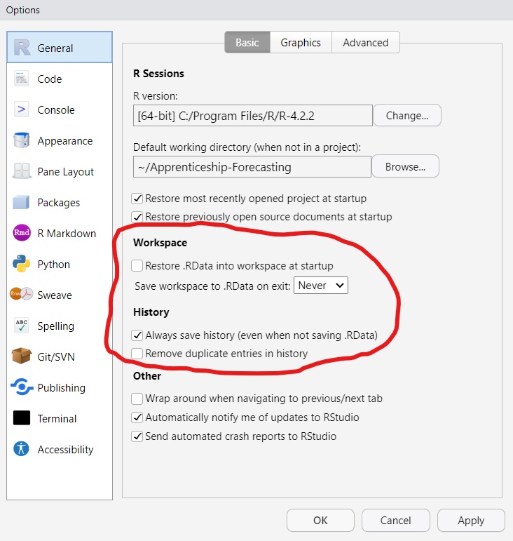
Session reloading from `.RData`

By default, RStudio will save and reload your R session from a .RData file. This discourages a reproducible workflow, so disable this feature! (RStudio -> Tools -> Global Options -> General)
Generally avoid saving R objects with save() and saveRDS(). It’s better to put a bit more work in to export to CSV, Excel or SQL.

Projects and filepaths

Create a new RStudio project for each new piece of work
A project is defined by the presence of a file with the .Rproj extension. This tells RStudio that everything in the folder is part of the project.
- Never use setwd() as this can result in code which other people can’t run. Instead, use relative filepaths.
Use a sub-directory R/ for your production R scripts
Write a README.md file for each project explaining its purpose and steps to get started using it
For long-term projects, or ones which are on hold, use {renv} to keep track of dependencies

fs::dir_tree("example-proj")

example-proj
├── example-proj.Rproj
├── in-development
│   ├── pupil-counts.sql
│   └── testing.R
├── R
│   ├── 01-import.R
│   ├── 02-tidy.R
│   ├── 03-model.R
│   └── 04-export.R
├── README.md
├── reports
│   └── analysis-report.qmd
└── SQL
    └── read-starts.sql

04. Some useful tools

`janitor::clean_names()`

clean_names() is a very quick and easy way to make syntactic column names. Use it!
Getting Title_Snake_Case is possible, but not obvious from the documentation
Renaming is lossy, so check the result

messy_df <- data.frame(
  pupilNumber      = 1:2, 
  `cost 2022`      = 1234, 
  `% totalFunding` = c(0.4, 0.6),
  `<50% funding`   = c(TRUE, FALSE), 
  check.names = FALSE
)

messy_df
#>    pupilNumber cost 2022 % totalFunding <50% funding
#>  1           1      1234            0.4         TRUE
#>  2           2      1234            0.6        FALSE

messy_df %>% 
  janitor::clean_names()
#>    pupil_number cost_2022 percent_total_funding x50_percent_funding
#>  1            1      1234                   0.4                TRUE
#>  2            2      1234                   0.6               FALSE

messy_df %>% 
  janitor::clean_names(case = "title", sep_out = "_")
#>    Pupil_Number Cost_2022 Percent_Total_Funding X50_Percent_Funding
#>  1            1      1234                   0.4                TRUE
#>  2            2      1234                   0.6               FALSE

`styler::style_file()`

{styler} is a powerful tool to use sparingly. Some reasonable use-cases:

Re-style a project you inherit
Re-style your own old projects after seeing this presentation

messy-code.R

#load packages
library(tidyverse);library(lubridate)

data_raw=read_csv(  "some_file.csv"  )

data_clean<-data_raw %>%
  mutate(Amount=Amount/sum(Amount),
    #Combine date parts into single column
    Date=make_date(Year,   Month,Day))%>%
    filter(
  # other years aren't relevant to analysis
          year(Date)==2020,
          Amount> 0.1
    )

ggplot2(data_clean,aes(Date,Amount))+geom_line()

styler::style_file("messy-code.R")

# load packages
library(tidyverse)
library(lubridate)

data_raw <- read_csv("some_file.csv")

data_clean <- data_raw %>%
  mutate(
    Amount = Amount / sum(Amount),
    # Combine date parts into single column
    Date = make_date(Year, Month, Day)
  ) %>%
  filter(
    # other years aren't relevant to analysis
    year(Date) == 2020,
    Amount > 0.1
  )

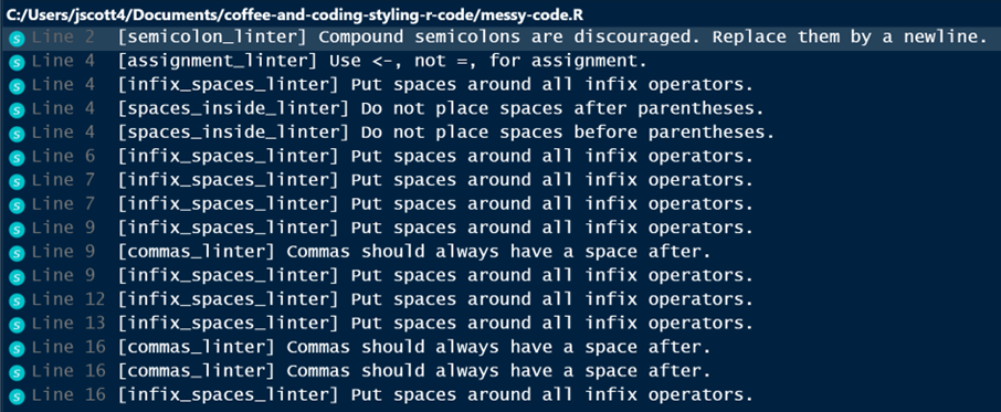
ggplot2(data_clean, aes(Date, Amount)) + geom_line()

`lintr::lint()`

{lintr} is similar to {styler}, but it tells you about issues instead of fixing them.

Good for maintaining already well-styled code, not so good for restyling old code
Highly customisable, e.g. if you want to relax/not apply some rules
RStudio’s UI lets you click through to address individual lints

messy-code.R

#load packages
library(tidyverse);library(lubridate)

data_raw=read_csv(  "some_file.csv"  )

data_clean<-data_raw %>%
  mutate(Amount=Amount/sum(Amount),
    #Combine date parts into single column
    Date=make_date(Year,   Month,Day))%>%
    filter(
  # other years aren't relevant to analysis
          year(Date)==2020,
          Amount> 0.1
    )

ggplot2(data_clean,aes(Date,Amount))+geom_line()

lintr::lint("messy-code.R")

Built-in tools in RStudio

Shortcut	Action
`Ctrl + I`	Correct indentation
`Alt + Ctrl + Shift + M`	‘Rename in scope’, e.g. change `myVar` to `my_var`
`Ctrl + Shift + F`	Find (and replace) throughout multiple files
`Ctrl + Shift + /`	Wrap long comments over multiple lines
`Alt + -`	Insert `<-` with the correct spacing
`Ctrl + Shift + M`	Insert `%>%` with the correct spacing
`Alt + Ctrl + Shift + R`	Inserts template function documentation
`Alt + click/drag`	Activate multiline cursor

Note: You can use Tools -> Keyboard Shortcuts Help for a full list of shortcuts

05. Resources

Resources

The Tidyverse style guide: https://style.tidyverse.org/
The Tidyverse design guide: https://design.tidyverse.org/
Workflow: code style (R for Data Science): https://r4ds.hadley.nz/workflow-style.html
The {styler} package: https://styler.r-lib.org/
The {lintr} package: https://lintr.r-lib.org/
The {usethis} package for project/package setup: https://usethis.r-lib.org/
The {devtools} package for package development: https://devtools.r-lib.org/
The {testthat} package for unit testing: https://testthat.r-lib.org/